Online Learning and Student Outcomes in Community Colleges (PPIC Publication)

Online Learning and Student Outcomes in Community Colleges (PPIC Publication):



Retention in California Community Colleges



'via Blog this'

The New CIO: Bruce Maas -- Campus Technology

The New CIO: Bruce Maas -- Campus Technology: "At UW-Madison, we have consciously separated the role of operations leader for IT from the CIO, to allow the CIO to work more strategically on mission-critical services. "



'via Blog this'

Discussion Section - Purdue OWL: Writing in Psychology: Experimental Report Writing

Purdue OWL: Writing in Psychology: Experimental Report Writing: "Begin by providing an interpretation of your results: what is it that you have learned from your research?
Discuss each hypotheses or research question in more depth.
Do not repeat what you have already said in your results—instead, focus on adding new information and broadening the perspective of your results to you reader.
Discuss how your results compare to previous findings in the literature. If there are differences, discuss why you think these differences exist and what they could mean.
Briefly consider your study's limitations, but do not dwell on its flaws.
Consider also what new questions your study raises, what questions your study was not able to answer, and what avenues future research could take in this area.
 "



'via Blog this'

Learning through social networking sites – the critical role of the teacher...: EBSCOhost

Learning through social networking sites – the critical role of the teacher...: EBSCOhost:



level of success of SNS learning activities can vary between classes depending on the way they are implemented.



social media



'via Blog this'

Pearson - Social Media for Teaching and Learning - Social Media Survey 2013

Pearson - Social Media for Teaching and Learning - Social Media Survey 2013: "
Annual survey of social media use by higher education faculty, 2013
Since 2009, Pearson has been researching faculty use of social media. As a learning company that promotes the effective use of technology, Pearson is acutely aware of how important it is to understand these emerging media, the opportunities they offer to higher education faculty, and how their adoption can evolve—and is evolving—teaching and learning in higher education. Pearson's ongoing collaboration with thought leaders from such organizations as the Babson Survey Research Group is enabling us to strengthen that understanding. As a reflection of our commitment to sharing our knowledge with the higher education community, the following pages contain the findings of our 2013 Social Media in Higher Education survey."



'via Blog this'

Multicollinearity

Multicollinearity: "How to detect multicollinearity?
Formally, variance inflation factors (VIF) measure how much the variance of the estimated coefficients are increased over the case of no correlation among the X variables. If no two X variables are correlated, then all the VIFs will be 1.
If VIF for one of the variables is around or greater than 5, there is collinearity associated with that variable.
The easy solution is: If there are two or more variables that will have a VIF around or greater than 5, one of these variables must be removed from the regression model.
 "



'via Blog this'

Multicollinearity

Multicollinearity: "How to detect multicollinearity?
Formally, variance inflation factors (VIF) measure how much the variance of the estimated coefficients are increased over the case of no correlation among the X variables. If no two X variables are correlated, then all the VIFs will be 1.
If VIF for one of the variables is around or greater than 5, there is collinearity associated with that variable.
The easy solution is: If there are two or more variables that will have a VIF around or greater than 5, one of these variables must be removed from the regression model.
 "



'via Blog this'

Regression with SPSS: Lesson 2 - Regression Diagnostics

Regression with SPSS: Lesson 2 - Regression Diagnostics: "The histogram shows some possible outliers.  We can use the outliers(sdresid) and id(state) options to request the 10 most extreme values for the studentized deleted residual to be displayed labeled by the state from which the observation originated.  Below we show the output generated by this option, omitting all of the rest of the output to save space.  You can see that "dc" has the largest value (3.766) followed by "ms" (-3.571) and "fl" (2.620)"



'via Blog this'

AndrewDart.co.uk : Reporting Multiple Regressions in APA format – Part One

AndrewDart.co.uk : Reporting Multiple Regressions in APA format – Part One: "Reporting Multiple Regressions in APA format – Part One

So this is going to be a very different post from anything I have put up before. I am writing this because I have just spent the best part of two weeks trying to find the answer myself without much luck. Sure I came across the odd bit of advice here and there and was able to work a lot of it out, but so many of the websites on this topic leave out a bucket load of the information, making it difficult to know what they are actually going on about. So after two weeks of wading through websites, texts book and having multiple meetings with my university supervisors, I thought I would take the time to write up some instructions on how to report multiple regressions in APA format so that the next poor sap who has this issue doesn’t have to waste all the time I did. If you have no interest in statistics then I recommend you skip the rest of this post."



'via Blog this'

Linear Regression Analysis in SPSS - Procedure, assumptions and reporting the output.

Linear Regression Analysis in SPSS - Procedure, assumptions and reporting the output.:


'via Blog this'

Introduction

Linear regression is the next step up after correlation. It is used when we want to predict the value of a variable based on the value of another variable. The variable we want to predict is called the dependent variable (or sometimes, the outcome variable). The variable we are using to predict the other variable's value is called the independent variable (or sometimes, the predictor variable). For example, you could use linear regression to understand whether exam performance can be predicted based on revision time; whether cigarette consumptions can be predicted based on smoking duration; and so forth. If you have two or more independent variables, rather than just one, you need to use multiple regression.

This "quick start" guide shows you how to carry out linear regression using SPSS, as well as interpret and report the results from this test. However, before we introduce you to this procedure, you need to understand the different assumptions that your data must meet in order for linear regression to give you a valid result. We discuss these assumptions next.

SPSStop ^

Assumptions

When you choose to analyse your data using linear regression, part of the process involves checking to make sure that the data you want to analyse can actually be analysed using linear regression. You need to do this because it is only appropriate to use linear regression if your data "passes" six assumptions that are required for linear regression to give you a valid result. In practice, checking for these six assumptions just adds a little bit more time to your analysis, requiring you to click a few more buttons in SPSS when performing your analysis, as well as think a little bit more about your data, but it is not a difficult task.

Before we introduce you to these six assumptions, do not be surprised if, when analysing your own data using SPSS, one or more of these assumptions is violated (i.e., not met). This is not uncommon when working with real-world data rather than textbook examples, which often only show you how to carry out linear regression when everything goes well! However, don’t worry. Even when your data fails certain assumptions, there is often a solution to overcome this. First, let’s take a look at these six assumptions:

• Assumption #1: Your two variables should be measured at the interval or ratio level (i.e., they are continuous). Examples of variables that meet this criterion include revision time (measured in hours), intelligence (measured using IQ score), exam performance (measured from 0 to 100), weight (measured in kg), and so forth. You can learn more about interval and ratio variables in our article:Types of Variable.
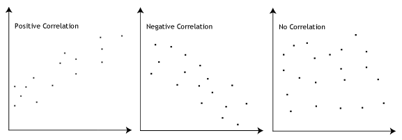
• Assumption #2: There needs to be a linear relationship between the two variables. Whilst there are a number of ways to check whether a linear relationship exists between your two variables, we suggest creating a scatterplot using SPSS, where you can plot the dependent variable against your independent variable, and then visually inspect the scatterplot to check for linearity. Your scatterplot may look something like one of the following:
  
  
  
  
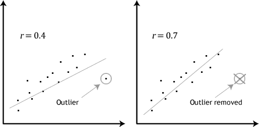
  If the relationship displayed in your scatterplot is not linear, you will have to either run a non-linear regression analysis or “transform” your data, which you can do using SPSS. In our enhanced guides, we show you how to: (a) create a scatterplot to check for linearity when carrying out linear regression using SPSS; (b) interpret different scatterplot results; and (c) transform your data using SPSS if there is not a linear relationship between your two variables.
• Assumption #3: There should be no significant outliers. Outliers are simply single data points within your data that do not follow the usual pattern (e.g., in a study of 100 students’ IQ scores, where the mean score was 108 with only a small variation between students, one student had a score of 156, which is very unusual, and may even put her in the top 1% of IQ scores globally). The following scatterplots highlight the potential impact of outliers:
  
  
  
  
  The problem with outliers is that they can have a negative effect on the regression equation that is used to predict the value of the dependent (outcome) variable based on the independent (predictor) variable. This will change the output that SPSS produces and reduce the predictive accuracy of your results. Fortunately, when using SPSS to run linear regression on your data, you can easily include criteria to help you detect possible outliers. In our enhanced linear regression guide, we: (a) show you how to detect outliers using "casewise diagnostics", which is a simple process when using SPSS; and (b) discuss some of the options you have in order to deal with outliers.
• Assumption #4: You should have independence of observations, which you can easily check using the Durbin-Watson statistic, which is a simple test to run using SPSS. We explain how to interpret the result of the Durbin-Watson statistic in our enhanced linear regression guide.
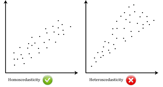
• Assumption #5: Your data needs to show homoscedasticity, which is where the variances along the line of best fit remain similar as you move along the line. Whilst we explain more about what this means and how to assess the homoscedasticity of your data in our enhanced linear regression line, take a look at the two scatterplots below, which provide two simple examples: one of data that meets this assumption and one that fails the assumption:
  
  
  
  When you analyse your own data, you will be lucky if your scatterplot looks like either of the two above. Whilst these help to illustrate the differences in data that meets or violates the assumption of homoscedasticity, real-world data is often a lot more messy. Therefore, in our enhanced linear regression guide, we explain: (a) some of the things you will need to consider when interpreting your data; and (b) possible ways to continue with your analysis if your data fails to meet this assumption.
• Assumption #6: Finally, you need to check that the residuals (errors) of the regression line are approximately normally distributed(we explain these terms in our enhanced linear regression guide). Two common methods to check this assumption include using either a histogram (with a superimposed normal curve) or by using a Normal P-P Plot. Again, in our enhanced linear regression guide, we: (a) show you how to check this assumption using SPSS, whether you use a histogram (with superimposed normal curve) or Normal P-P Plot; (b) explain how to interpret these diagrams; and (c) provide a possible solution if your data fails to meet this assumption.

You can check assumptions #2, #3, #4, #5 and #6 using SPSS. Assumptions #2 and #3 should be checked first, before moving onto assumptions #4, #5 and #6. We suggest testing these assumptions in this order because it represents an order where, if a violation to the assumption is not correctable, you will no longer be able to use a single linear regression (although you may be able to run another statistical test on your data instead). Also, you check assumptions #4, #5 and #6 at the same time as running the linear regression procedure in SPSS, so it is easier to deal with these after checking assumptions #2 and #3. Just remember that if you do not run the statistical tests on these assumptions correctly, the results you get when running a linear regression might not be valid. This is why we dedicate a number of sections of our enhanced a linear regression guide to help you get this right. You can find out about our enhanced content as a whole here, or more specifically, learn how we help with testing assumptions here.

In the section, Procedure, we illustrate the SPSS procedure to perform a linear regression assuming that no assumptions have been violated. First, we introduce the example that is used in this guide.

A salesperson for a large car brand wants to determine whether there is a relationship between an individual's income and the price they pay for a car. Therefore, the individual’s "income" is the independent (predictor) variable and the "price" they pay for a car is the dependent (outcome) variable. The salesperson wants to use this information to determine which cars to offer potential customers in new areas where average income is known.

SPSStop ^

Setup in SPSS

In SPSS, we created two variables so that we could enter our data: Income (the independent/predictor) variable, and Price (the dependent/outcome variable). It can also be useful to create a third variable, caseno, to act as a chronological case number. This third variable is used to make it easy for you to eliminate cases (e.g., significant outliers) that you have identified when checking for assumptions. However, we do not include it in the SPSS procedure that follows because we assume that you have already checked these assumptions. In our enhanced linear regression guide, we show you how to correctly enter data in SPSS to run a linear regression when you are also checking for assumptions. You can learn about our enhanced data setup content here. Alternately, we have a generic, "quick start" guide to show you how to enter data into SPSS, available here.

SPSStop ^

Test Procedure in SPSS

The five steps below show you how to analyse your data using linear regression in SPSS when none of the six assumptions in the previous section, Assumptions, have been violated. At the end of these five steps, we show you how to interpret the results from your linear regression. If you are looking for help to make sure your data meets assumptions #2, #3, #4, #5 and #6, which are required when using linear regression, and can be tested using SPSS, you can learn more in our enhanced guide here.

• Click Analyze > Regression > Linear... on the top menu.
  
  

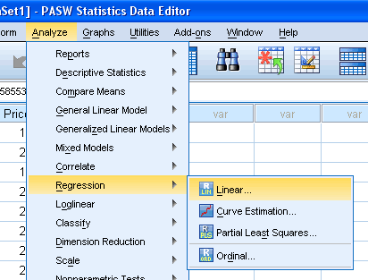
  Published with written permission from SPSS Inc., an IBM Company.
• You will be presented with the following dialog box:
  
  

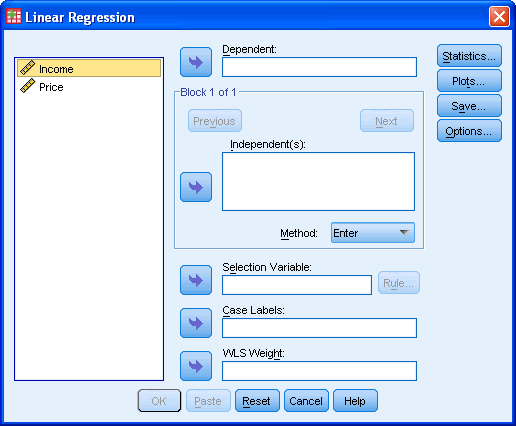
  Published with written permission from SPSS Inc., an IBM Company.
• Transfer the independent (predictor) variable, Income, into the Independent(s): box and the dependent (outcome) variable,Price, into the Dependent: box. You can do this by either drag-and-dropping or by using the  buttons.
  
  

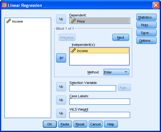
  Published with written permission from SPSS Inc., an IBM Company.
• You now need to check four of the assumptions discussed in the Assumptions section above: No significant outliers (assumption #3); independence of observations (assumption #4); homoscedasticity (assumption #5); and normal distribution of errors/residuals (assumptions #6). You can do this by using the  and  features, and then selecting the appropriate tick boxes within these two dialogue boxes. In our enhanced linear regression guide, we show you which options to select in order to test whether your data meets these four assumptions.
• When you have ticked the relevant options in the  and  option boxes above, click the  button.
• top ^

Output of Linear Regression Analysis

SPSS will generate quite a few tables of output for a linear regression. In this section, we show you only the three main tables required to understand your results from the linear regression procedure, assuming that no assumptions have been violated. A complete explanation of the output you have to interpret when checking your data for the six assumptions required to carry out linear regression is provided in our enhanced guide here. This includes relevant scatterplots, histogram (with superimposed normal curve) and Normal P-P Plot, and casewise diagnostics and Durbin-Watson statistic tables. Below, we focus on the results for the linear regression analysis only.

The first table of interest is the Model Summary table. This table provides the R and R² value. The R value is 0.873, which represents the simple correlation. It indicates a high degree of correlation. The R² value indicates how much of the dependent variable, "price", can be explained by the independent variable, "income". In this case, 76.2% can be explained, which is very large.

Published with written permission from SPSS Inc., an IBM Company.

The next table is the ANOVA table. This table indicates that the regression model predicts the outcome variable significantly well. How do we know this? Look at the "Regression" row and go to the Sig. column. This indicates the statistical significance of the regression model that was applied. Here, p < 0.0005, which is less than 0.05, and indicates that, overall, the model applied can statistically significantly predict the outcome variable.

Published with written permission from SPSS Inc., an IBM Company.

The table below, Coefficients, provides us with information on each predictor variable. This gives us the information we need to predict price from income. We can see that both the constant and income contribute significantly to the model (by looking at the Sig. column). By looking at the B column under the Unstandardized Coefficients column, we can present the regression equation as:

Price = 8287 + 0.564(Income)

Published with written permission from SPSS Inc., an IBM Company.

If you are unsure how to interpret regression equations, or how to use them to make predictions, we discussed this in our enhanced linear regression guide. We also show you how to write up the results from your assumptions tests and linear regression output if you need to report this in a dissertation/thesis, assignment or research report. We do this using the Harvard and APA styles. You can learn more about our enhanced content here.

We also show you how to perform a linear regression analysis in SPSS here.

From Laerd

Linear Regression Analysis in SPSS - Procedure, assumptions and reporting the output.

Linear Regression Analysis in SPSS - Procedure, assumptions and reporting the output.:



'via Blog this'

MANOVA

MANOVA:



'via Blog this'

Using SPSS for t-Tests

Using SPSS for t-Tests:



'via Blog this'

How do I report paired samples T-test data in APA style?

How do I report paired samples T-test data in APA style?:



'via Blog this'

Three things to report 

You will want to include three main things about the Paired Samples T-Test when communicating results to others.

1. Test type and use

You want to tell your reader what type of analysis you conducted. If you don’t, your results won’t make much sense to the reader. You also want to tell your reader why this particular analysis was used. What did your analysis tests for?

Example

You can report data from your own experiments by using the template below.

“A paired-samples t-test was conducted to compare (your DV measure) _________ in (IV level / condition 1) ________and (IV level / condition 2)________ conditions.”

If we were reporting data for our example, we might write a sentence like this.

“A paired-samples t-test was conducted to compare the number of hours of sleep in caffeine and no caffeine conditions.”

2. Significant differences between conditions

You want to tell your reader whether or not there was a significant difference between condition means. You can report data from your own experiments by using the template below.

“There was a significant (not a significant) difference in the scores for IV level 1 (M=___, SD=___) and IV level 2 (M=___, SD=___) conditions; t(__)=___, p = ____”

Just fill in the blanks by using the SPSS output

Let’s start by filing in the Mean and Standard Deviation for each condition.

Now we’ll finish up by filling in the values related to the paired T-Test. Here we enter the degrees of freedom (df), the t-value (t), and the Sig. (2-tailed) value (often referred to as the p value).

 

Once the blanks are full…

You have a sentence that looks very scientific but was actually very simple to produce.

“There was a significant difference in the scores for caffeine (M=5.4, SD=1.14) and no caffeine (M=9.4, SD=1.14) conditions; t(4)=-5.66, p = 0.005.”

3. Report your results in words that people can understand

Since it might be hard for someone to figure out what that sentence means or how it relates to your experiment, you want to briefly recap in words that people can understand. Try to imagine trying to explain your results to someone who is not familiar with science. In one sentence, explain your results in easy to understand language.

Example

You might write something like this for our example.

“These results suggest that caffeine really does have an effect hours slept. Specifically, our results suggest that when humans consume caffeine, the number of hours they sleep decreases”

You could have also written the following sentence.

“These results suggest that caffeine really does have an effect hours slept. Specifically, our results suggest that when humans consume less caffeine, the number of hours they sleep increases.”

Both sentences are so much easier to understand than the scientific one will all of the numbers in it.

Let’s see how this looks all together

When you put the three main components together, results look something like this.

“A paired-samples t-test was conducted to compare hours of sleep in caffeine and no caffeine conditions. There was a significant difference in the scores for caffeine (M=5.4, SD=1.14) and no caffeine (M=9.4, SD=1.14) conditions; t(4)=-5.66, p = 0.005. These results suggest that caffeine really does have an hours slept. Specifically, our results suggest that when humans consume caffeine, the number of hours they sleep decreases.”

Looking good!